NOTE: This CRISPR exercise recreates experiments that resulted in the 2020 Nobel Prize in Chemistry*. A separate ATTR exercise recreates experiments that resulted in the first successful use of CRISPR for in vivo therapy of a genetic condition. The procedure for Part 4 of this CRISPR exercise is used as an example in the DNA digestion & electrophoresis tutorial.
Update 7/2/23: A mobile version of Part 4 is now available, linking to a video of Case It v705 running the procedure described in Part 4 of this exercise.
*Update 10/7/20: Jennifer Doudna and Emmanuelle Charpentier have been awarded the Nobel Prize in Chemistry for the research paper that is the basis for this CRISPR exercise. Note that Part 4 covers the key experiment (as described by Jennifer Doudna in this video ). Some earlier practical applications made possible by this pioneering research are linked here. Many additional applications have appeared since these were published.
Goal of this exercise: Use Case It v7.0.5 to recreate and analyze experiments that first demonstrated the function of Cas9, an enzyme that plays a fundamental role in CRISPR applications such as gene editing. Considered “one of the most significant discoveries in recent history“, these experiments are from Jinek et al. 2012 and its Supplement, organized into four parts. Part 1 covers experiments on the ability of Cas9 to function as a programmable restriction enzyme, using both plasmid and oligonucleotide DNA. An answer key is available to instructors upon request (contact mark.s.bergland@uwrf.edu).
Part 1: Experiments on site-specific actions of Cas9
Part 2: Experiments with mutations to determine Cas9 gene function
Part 3: PAM requirements and the sensitivity of Cas9 to mismatch
Part 4: Experiments targeting GFP gene sequences
Background
Before going through the steps below, it is highly recommended that you read through this brief introduction to CRISPR (part of the ATTR exercise), then use the back arrow of your browser to return here.
It would also be very helpful to view this video introduction to CRISPR technology by Jennifer Doudna and read the interview with Martin Jinek on the Nobel Prize-winning research that is the basis for this CRISPR exercise.
Organization of Part 1
Numbered steps below include links to images of the Case It simulation. If images do not appear sharp, use the Control (or Command) keys in conjunction with the plus and minus keys to change image size. Informational notes and questions are included in blue and yellow boxes, with text in italics.
________________________________
Step 1: Download Case It v7.0.4 – earlier versions will not work with this exercise.
Steps 2-16: Plasmid experiments based on Fig 1A of Jinek et al 2012.
Steps 17-29: Oligonucleotide experiments based on Fig 1B and 1D.
Step 30: Repeating experiments with a different protospacer (Figs S3 and S5 of the Supplement).
**Note to instructors: The first section of Part 1 (through Step 16) covers preliminary experiments and also serves as an introduction to Case It software. The key experiment from Jinek et al. 2012 is covered in Part 4. Although Part 4 can serve as a stand-alone exercise, it is best to have students go through the first section of Part 1 (just to get familiar with the software) before skipping to Part 4. Parts 2 and 3 cover additional experiments but are not necessary for student understanding and analysis of Part 4.
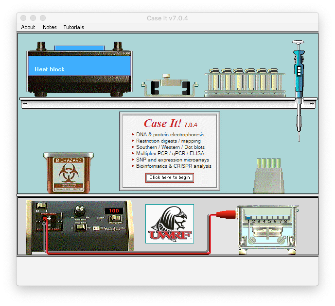
1. If you have not already done so, download Case It v7.0.5 and follow the instructions on the PDF file containing the download link. Earlier versions of the Case It software (except Case It v7.0.4) do not have CRISPR capability and thus will not work with this exercise. If you are unsure which version you have, the version number is part of the executable name and can also be found on the splash screen when the software first opens. It should look like this, with the UWRF logo at bottom center.
Note: If you are going to use Case It on a Mac, the downloaded zip file must first be removed from quarantine by running a single line in Terminal window of the Mac. The file can then be unzipped and Case It will run on any Mac exactly as it does on Windows. See the PDF file containing the download link (available from the Download page) for detailed instructions.
Recommended browser: Firefox is preferred if you are using Windows, as images are clearer compared to Chrome or Edge. On Macs, any browser can be used.
The goal of the first series of steps (2-16) is to determine if Cas9 can be “programmed” to cut a particular location on a plasmid. This will be tested by exposing the plasmid to Cas9 in the presence of two different guide RNAs (see note below*). One of these includes the recognition site for ‘protospacer 2’ (ps2), whereas the other includes the recognition site for ‘protospacer 1’ (ps1). The plasmid used in this experiment was constructed to include only the ps2 sequence.
Exercise: Based on the information in the gray box above, formulate a hypothesis for this particular experiment. Remember that a hypothesis is in the form of a statement, not in the form of a question.
*Note: The ‘Cas9 enzyme’ files used in this exercise only contain the protospacer recognition sequences, as that is all the simulation requires to find these sites on a DNA sequence. In reality, tracrRNA and crRNA would have to be present (along with Cas9), associated together by complementary base pairing (this ‘dual guide RNA’ association is called the crRNA : tracrRNA duplex in Jinek’s paper). For a visual representation, see Fig 1E of Jinek et al. 2012, and also the introduction to CRISPR in Part 1 of the ATTR exercise.
Later in the experimental procedure, this duplex was modified by shortening crRNA and tracrRNA and linking it together into a single guide RNA, called ‘chimeric RNA’ in Jinek’s paper. For a visual representation, see Fig 5A of Jinek et al. 2012.
Jinek used the terms complementary and non-complementary to differentiate between the strands of the DNA molecule, so that is the terminology used here. They are now called the target strand and the non-target strand. Guide RNA binds directly to the target strand, and the PAM sequence is located on the non-target strand (see the introduction to CRISPR).
For this exercise, we are also assuming that magnesium is present for all lanes of the gel. The original experiment included lanes with and without magnesium, to test the effect of magnesium on Cas9 function, but that aspect of the experiment is not covered here.
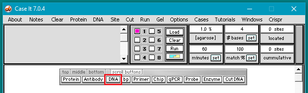
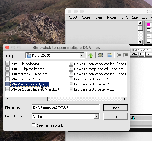
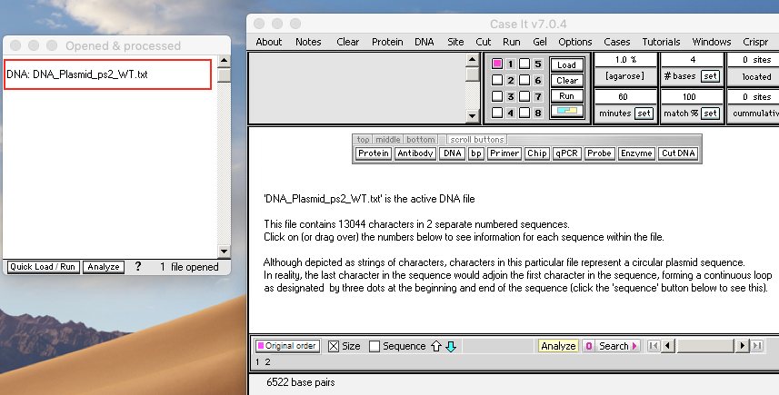
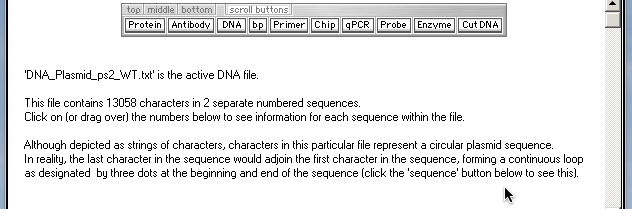
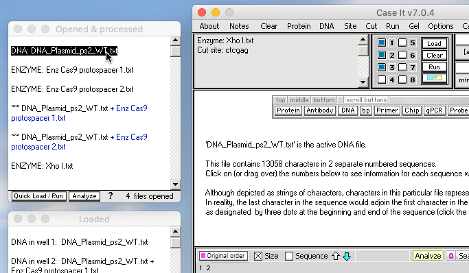
2. Use the DNA button on the silver button bar and navigate to the CRISPR data folder which is inside the Case It v7.0.4 folder. Open the folder named ‘Fig 1, S3, S5’ and double-click on the file ‘DNA Plasmid ps2 WT.txt’ that is inside that folder. The filename will appear in the Opened & Processed (O&P) window to the left of the main window.
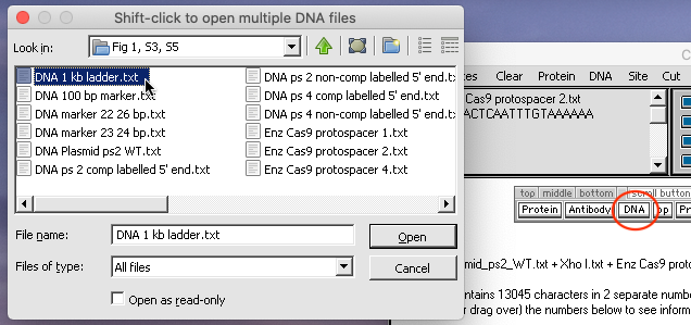
Note: If the the arrangement of files within the folder does not match that of the linked image in Step 2 above, click the List view button in the upper right-hand corner of the dialog box.
If you need more room on your screen, close the Sequence Analysis and Help windows to the right of the main window, as those windows will not be needed for this exercise.
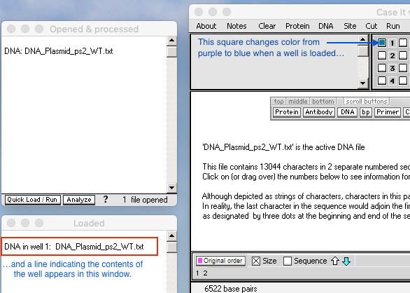
Plasmid DNA has a special file format, as indicated by this message that appears when a plasmid sequence is opened. If the word ‘plasmid’ is in the filename, the sequence will be treated as a circular loop of DNA. For this particular file, ‘ps2’ indicates that the plasmid contains the protospacer 2 sequence, and ‘WT’ stands for ‘wild type’.
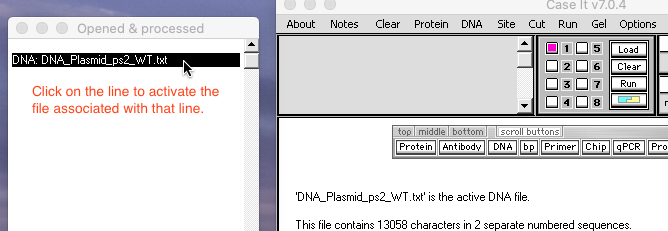
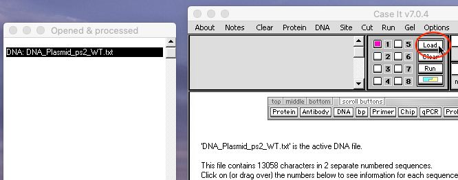
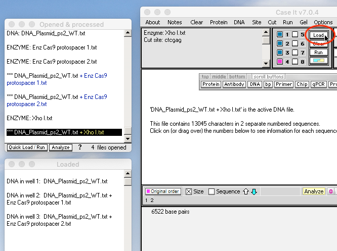
3. Click on the filename in the O&P window to activate, it then click the Load button to load the plasmid sequence into the first well. Note that the square associated with well 1 has changed color and the contents of the well appears as a line in the Loaded window.
Important: Before loading a well, make sure to click a line in the Opened & Processed (O&P) window to activate that file for loading, before clicking the Load button. This will ensure that the correct information appears in the Loaded window, indicating the contents of that well.
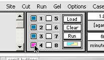
To select a well, click on its associated white square, and the square will turn purple indicating that it is ready for loading. When the Load button is clicked, the square turns blue. The first well square is selected by default when the program opens. For wells 2-7, it is necessary to click on a well square to select it, before clicking the Load button to load one of those wells.
Question: What is a ‘wild type’ plasmid, and why should this undigested plasmid be loaded into a well?
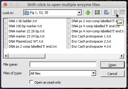
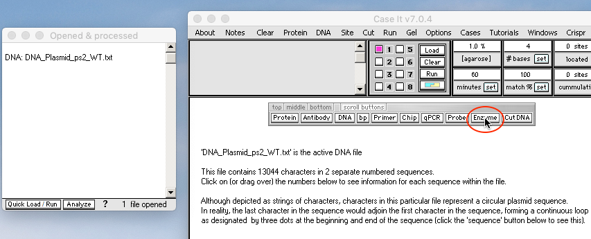
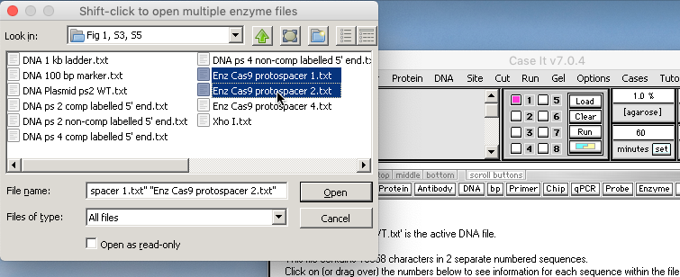
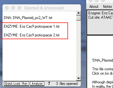
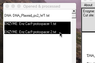
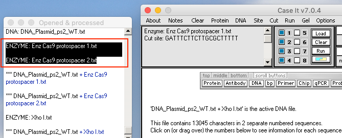
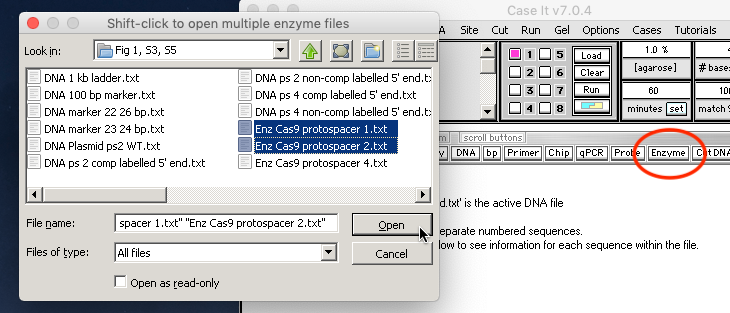
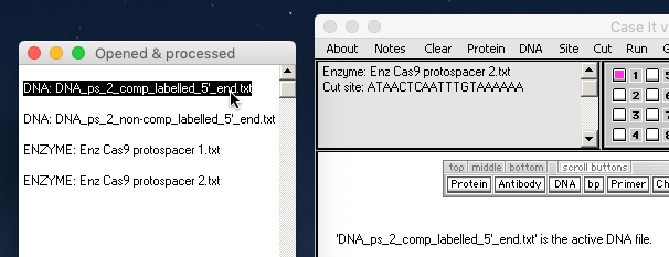
4. Click the Enzyme button and shift-click* to select the files ‘Enz Cas9 protospacer 1.txt’ and ‘Enz Cas9 protospacer 2.txt’, then open them (see note below). Two new lines will appear in the Opened & processed (O&P) window.
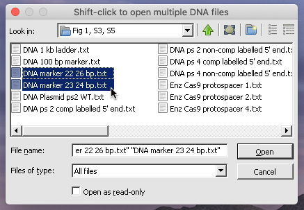
*Throughout these exercises the ‘shift-click’ technique is used to select multiple lines in a dialog box or window. To do this, click on a line and then hold down the shift key before clicking on another line. This will select (highlight) those lines and any lines in between. You can then click on the Open button to open the selected files. A quicker way to open files is to click on the first line, then double-click rather than single-click on another line with the shift key still held down. This will open all selected files without having to click the Open button.
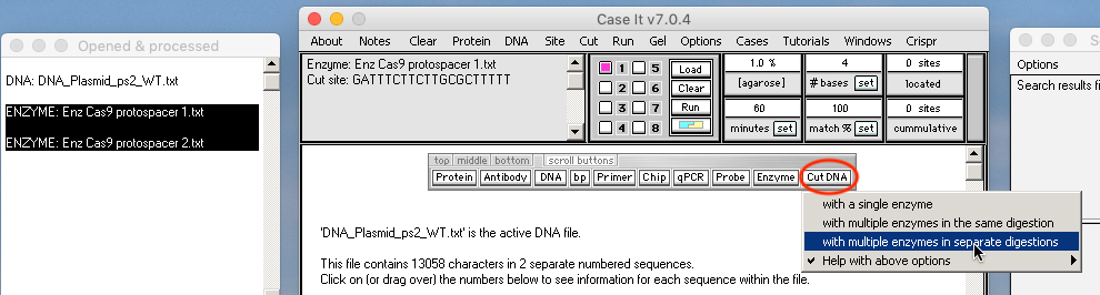
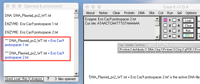
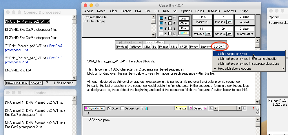
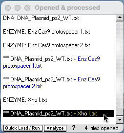
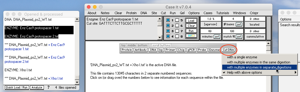
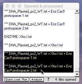
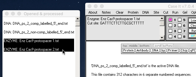
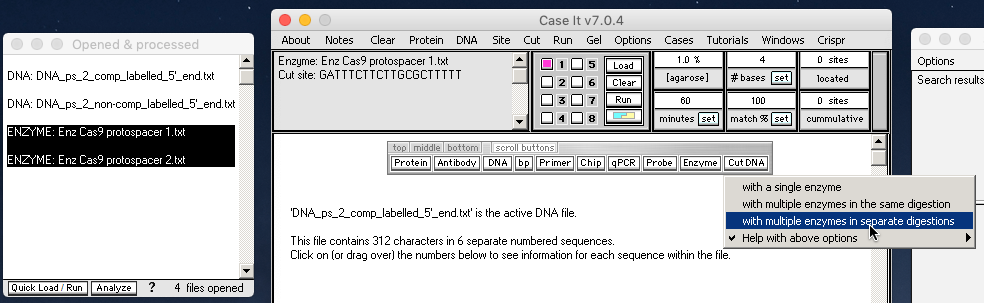
5. Shift-click to select (highlight) both enzymes in the Opened & Processed (O&P) window, then click the Cut DNA button on the silver button bar, and select ‘with multiple enzymes in separate digestions’ from the drop-down menu. Note that two new lines appear in the O&P window, representing the digested plasmids. You can tell this because of the asterisks (***) that precede each line.
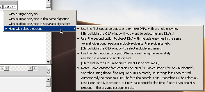
Note: When asterisks (***) precede a line in the O&P window, that line represents a DNA sample exposed to one or more restriction enzymes. It doesn’t necessarily mean that the DNA has been cut by those enzymes, because the enzyme(s) in question may or may not be able to cut a particular DNA sequence. For the purpose of this exercise, the word “digested” really means “exposed to”. Following this same reasoning, the ‘Cut DNA’ button should have been named the ‘attempt to cut DNA’ button, but that would have been awkward and wouldn’t have fit on the silver button bar! The Help menu of the ‘Cut DNA’ button explains when to use a particular option for exposing one or more DNA samples to one or more restriction enzymes.
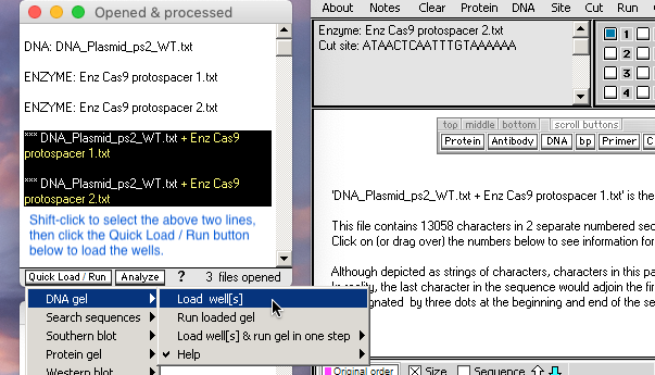
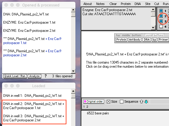
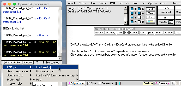
6. Shift-click to highlight the two *** DNA lines, and then use the Quick Load / Run button and select ‘DNA gels => Load well[s]‘ to automatically load wells two and three with these sequences. The Quick Load / Run button is located at the bottom of the Opened & processed window.
Labels for those two wells appear in the Loaded window, and the squares associated with wells 2 and 3 change color from purple to blue.
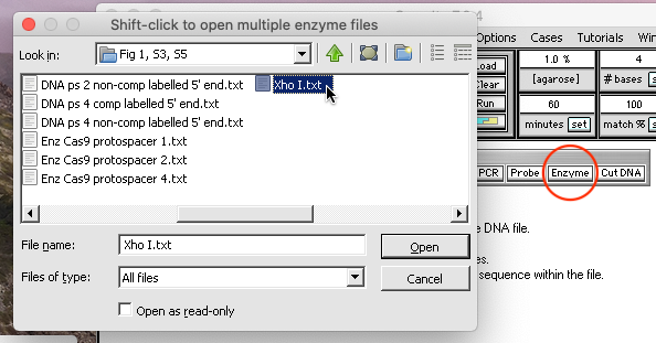
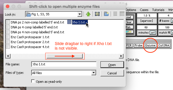
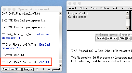
7. Click the enzyme button on the silver button bar and double-click on the enzyme ‘Xhol.txt’ to open that file. (if that filename is not visible, slide the dragbar of the dialog box to the right to see it.)
Note: Another way to access this enzyme is to click the blue/yellow button and select Xhol from the drop down menu. This menu shows the double-stranded configuration of this and other restriction enzymes.
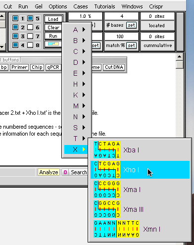
Questions: What type of cut does Xhol create? Why are these types of enzyme sites often found in constructed plasmids? (Click the link in the note above to help answer the first question).
8. Click the first line in the O&P window to make the undigested WT plasmid the active DNA file, and then click the Cut DNA button and select ‘with a single enzyme‘ from the drop-down menu. A new line with *** appears in the O&P window, indicating that the line represents the original WT plasmid file digested by XhoI. Click this line to activate it before going to the next step.
Important: Always click on the DNA file of interest to activate it, before doing anything else.
Question: Why would you want to digest the WT plasmid DNA with Xhol at this stage in the experimental procedure?
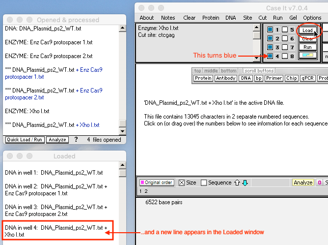
9. Click the white button next to the ‘4’ to select well four for loading, then click the Load button. The button turns blue, and a new line appears in the Loaded window indicating that the Xhol-digested plasmid has been loaded into well 4.
10. Click on the last line in the O&P window to activate the Xhol-digested plasmid, then shift-click in the O&P window to highlight and activate the two Cas9 enzyme files.
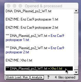
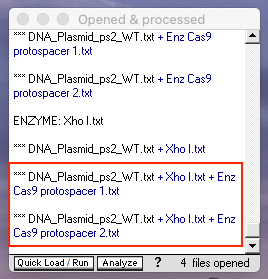
Click the Cut DNA button and select ‘with multiple enzymes in separate digestions‘. Two new ***lines appear in the O&P window, each representing the WT plasmid digested by Xhol and one of the two Cas9 enzymes.
Question: Why would you want to expose the Xhol-digested plasmid to two different Cas9 enzymes?
11. Shift-click to highlight the two new lines and then use the Quick Load / Run button to automatically load wells five and six with these sequences.
12. Click the DNA button and select ‘DNA_1_kb_ladder.txt‘.
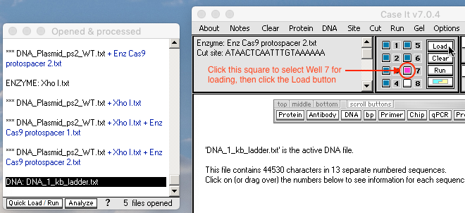
13. Click the white button next to the ‘7’ to select well seven for loading, then click the Load button. The button turns blue, and a new line appears in the Loaded window.
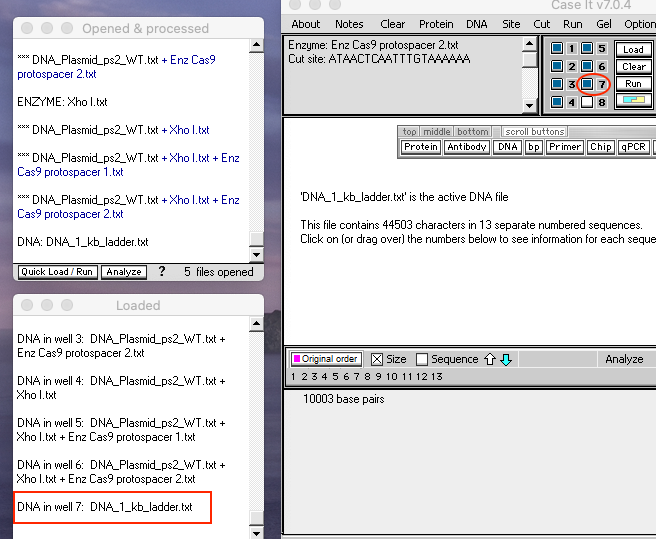
Question: What is the purpose of a DNA ladder on a gel?
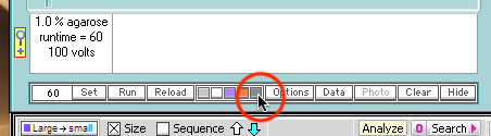
14. Click the Run button to run the gel. The gel appears with bands that are barely visible. To make them easier to see, click the black button under the gel. This gives an appearance similar to that of the gel in Fig 1A of Jinek et al. 2012 (rotated 90 degrees from Fig 1A).
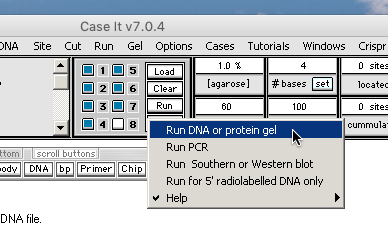
Note: You can change the appearance of the gel by clicking other colored buttons under the gel, to mimic methods of staining, etc. If you click a band, the size is shown in the lower field of the Data Screen, and you can click checkboxes to toggle back and forth between size and sequence. Although it is not necessary for this particular gel, you can also reload and re-run gels at different timer settings (to do this, change the number that appears in the white box below the gel, click Set to change the gel timer, then click the Run button below the gel).
15. There are three options for saving your gel results, including information about what is loaded into each well. The first option is to include the Loaded window in a screen shot* of the gel. If you do this, make sure that all information is shown in the Loaded window, by expanding it vertically if necessary.
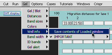
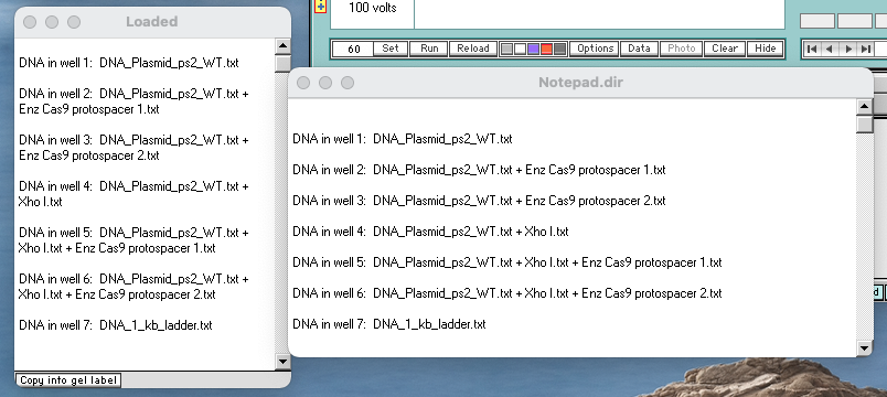
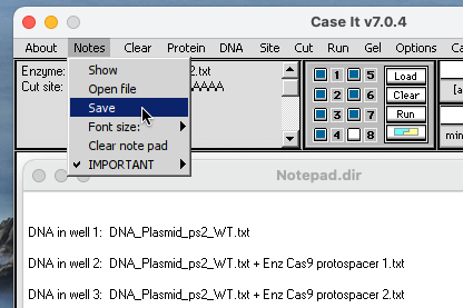
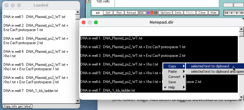
A second option is to copy the contents of the Loaded window into the Note Pad, via a command in the Gel menu. The Notepad will appear with the information copied into it. Drag the lower edge downward so that all of the information is visible, then include that in a screen shot instead of the Loaded window. Text in the Note Pad can also be saved as a text file or copied from the Notepad (via right-clicking) and then pasted into another application. If you save it as a text file, be sure to rename the file every time you save it. Otherwise, it may not save properly.
A third option is described in the Note in the blue field below. Although this enables the information to appear in the label right below the gel, the relatively small size of the label limits the amount of information it can hold, so it is better (and faster) to use one of the other options above.
*How to take screenshots:
Snipping Tool (and the newer Snip & Sketch) allows you to capture portions of your screen on Windows computers. Open Snipping Tool, click New, and drag the screen to capture an image of the Loaded window along with the gel. The image can then be saved in various formats, although .png is preferred.
To use Snip & Sketch, hold down the Windows key, the Shift key and the letter S simultaneously, then drag to select what you want to capture. Click on the Notifications button on the extreme right end of the task bar, then click on the Snip saved to clipboard image of your screen capture. You’ll then be able to save the image, in the preferred .png format.
For the Mac, one way to capture the screen is to use the Preview application. Open the application and select ‘Take Screenshot’ from the File menu. There are three options: From Selection, From Window, and From Entire Screen. The first option is the easiest way to capture an image of the Loaded window along with the gel (drag the screen to capture an image). The image can then be saved as a .png file. On Macs, the Screenshot app (formerly Grab) can also be used to capture the screen.
Note: Another way to label the gel is by transferring information from the Loaded window to the label beneath the gel. To do this, select characters and click the ‘Copy into gel label’ button. The characters automatically appear in the label beneath the gel. Repeat this process for the information for well two. Note that there are extraneous characters that can be removed without changing meaning. Edit these characters to allow more room on the gel label. Repeat this process so that all well label information in on the gel label. You can also select characters and right-click to copy them to the clipboard, then click in the gel label and right-click to paste the selected characters. Always select the minimum number of characters necessary to convey meaning, as space is limited on the gel label.
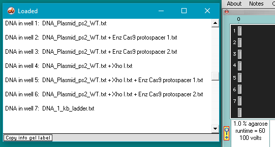
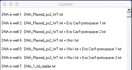
16. Your Loaded window should look like the one below (the left edge was dragged to expand the window). Compare your results with Figure 1A of Jinek et al. 2012, then answer the questions below:
Questions:
A. Which lanes in Fig 1A correspond to lanes in your gel, in terms of the experimental procedure used? Before answering, see the blue note just above Step 2, as not all lanes in Fig 1A were recreated on your gel.
B. For the ‘circular’ plasmid lanes on the left in Fig 1A, only one has a single band, whereas the others have two bands. Why is that?
C. Although somewhat difficult to see in Fig 1A, one of the ‘linearized’ lanes has two bands, whereas the others have a single band. Why is that? (note that it is easier to see this on the virtual gel)
D. Compare the minus and plus signs associated with various lanes in Fig 1A, especially in regard to crRNA-sp1 and crRNA-sp2, keeping in mind information in the blue note just above Step 2. What conclusions can you come to based on these comparisons?
E. Although not part of our virtual experiment, the original experiment also tested the effect of magnesium on the action of Cas9. Looking at the actual gel in Fig 1A, is magnesium necessary for proper Cas9 function?
The next series of steps will analyze site recognition features of Cas9 in greater detail using oligonucleotide DNA rather than plasmid DNA. The goal is to compare how Cas9 cuts the complementary versus the non-complementary strand of the oligonucleotide DNA molecule, by determining precisely where the cuts occur on these two strands.
Question: In general, what is an oligonucleotide? What is the literal meaning of the prefix ‘oligo’? Can you give another example of the use of this prefix in biology?
Note: The steps below are less detailed than those given previously, as it is assumed that you are now familiar with opening files, loading, and running gels. If not, please review Steps 1-16 above before continuing.
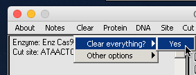
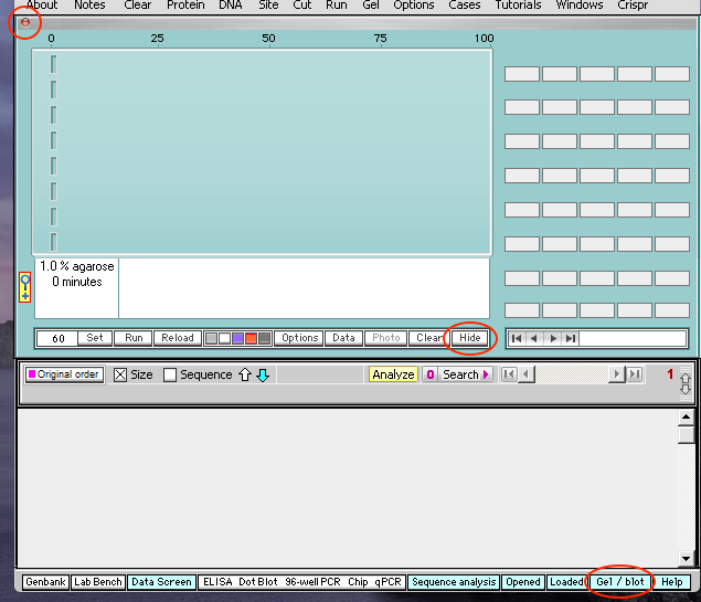
17. Use the Clear menu to ‘Clear everything‘, and hide the cleared gel by either (1) clicking the small red button in the upper left-hand corner of the gel, (2) clicking the ‘hide’ button in the lower left-hand corner of the gel, or (3) clicking the ‘Gel / blot’ button at the bottom of the Data Screen. That button can be used to both hide and show the gel.
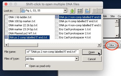
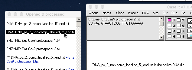
18. Use the DNA menu to open ‘DNA ps 2 comp labelled 5′ end.txt’ and ‘DNA ps 2 non-comp labelled 5′ end.txt’ inside the folders CRISPR data => ‘Fig 1, S3, S5’. Caution: Don’t open the ‘ps 4’ files by mistake, as they are located right next to the ‘ps2‘ files in the same folder. The ‘ps 4’ files won’t be used until Step 30 below, when the experiment is repeated using protospacer 4.
Note: These two files represent oligonucleotides containing protospacer 2, radiolabeled on the 5′ ends of the complementary and non-complementary strands (Figs 1B-E of Jinek et al. 2012). Radiolabeling is the process of adding a radioactive isotope to the end of a DNA molecule so that only fragments incorporating those radiolabels show up on an x-ray gel.
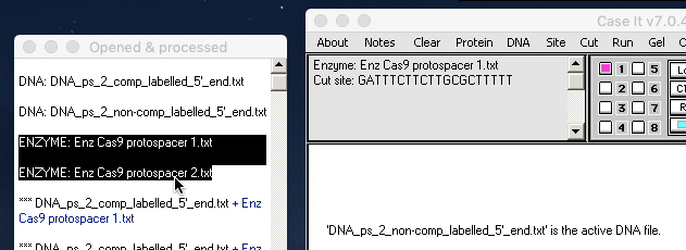
19. Use the Enzyme button to open the files ‘Enz Cas9 protospacer 1.txt’ and ‘Enz Cas9 protospacer 2.txt’.
20. Make ‘DNA ps 2 comp labelled 5′ end.txt’ the active DNA file by clicking on that line in the Opened & processed (O&P) window.
21. Shift-click to select the two Cas9 enzymes.
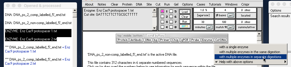
22. Click the Cut DNA button and select ‘with multiple enzymes in separate digestions‘. Two new lines (with ‘***’ prefixes) will appear in the O&P window, representing the digested DNA samples.
23. Make ‘DNA ps 2 non-comp labelled 5′ end.txt’ the active DNA file by clicking on that line in the Opened & processed (O&P) window.
24. Shift-click to select the two Cas9 enzymes.
25. Click the Cut DNA button and select ‘with multiple enzymes in separate digestions‘. Two new lines (with ‘***’ prefixes) will appear in the O&P window, representing the digested DNA samples.
26. Use the DNA button to open the files ‘DNA marker 22 26 bp.txt’ and ‘DNA marker 23 24 bp.txt‘. These files contain sequences of known size. The first file contains two sequences (22 bp and 26 bp), and the second contains two sequences (23 bp and 24 bp). These ‘markers’ serve as reference points for determining the sizes of bands in other lanes of the gel.
27. Use the DNA menu (located at the top of the Data Screen) to change the agarose concentration from the default value of 1.0 % to a value of 2.0 %. This new value will appear in the agarose field of the Data Screen.
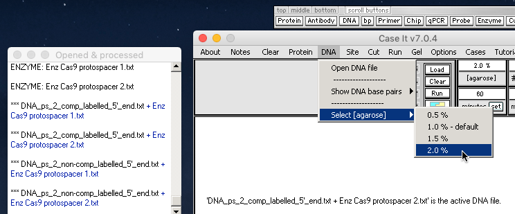
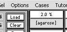
Question: Why would we want to increase the agarose concentration for this particular gel run, considering the relatively small size of the oligonucleotides that we are dealing with?
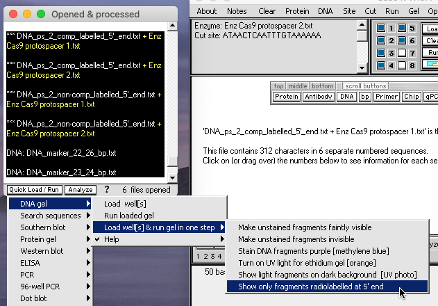
28. Shift-click to select the four digested DNA samples, along with the two marker files. Then click the Quick Load / Run button, and select DNA gel => Load well[s] & run gel in one step => Show only fragments radiolabelled at 5′ end from the drop-down menu.
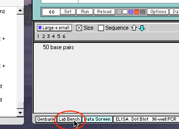
When the gel appears, you can click on bands to determine size, make bands narrower, and magnify the gel as discussed below.
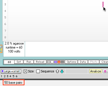
Note: Click on bands on the virtual gel to determine their size, which will appear in the field on the Data Screen below the gel. Make sure to click slowly, and get your cursor right on top of the gel. If you do this correctly an hour-glass cursor will briefly appear and the clicked band will turn red. In this example, the band is 50 bp in size. Change the band back to its original color by clicking anywhere in the lane associated with that band.
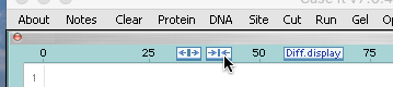
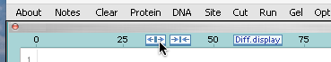
Since there are multiple bands in some of the lanes, it will be easier to distinguish them (and compare them with the actual gels) if you make the bands narrower. To do this, click the button with the inward-pointing arrows at the top of the gel. To revert to the original band widths, click the button with outward-pointing arrows. Note that wider bands are easier to click on than narrow bands.
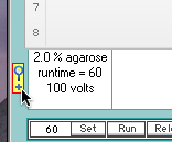
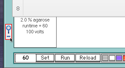
It may also be helpful to magnify the gel by clicking the magnifying glass icon. Click the icon again to return the gel to its original size. If the magnified gel is dragged by its upper edge, it will automatically return to its original size, so you will have to click the icon again once the gel has been dragged to a new position.
………………………………………………………………….
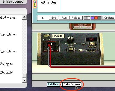
=> If dotted boxes appear around menu names at the top of the Data Screen, click the Lab Bench button at the bottom of the screen to go to a virtual laboratory bench, and then immediately click the Data Screen button to go back. The dotted boxes on the Data Screen will have disappeared.
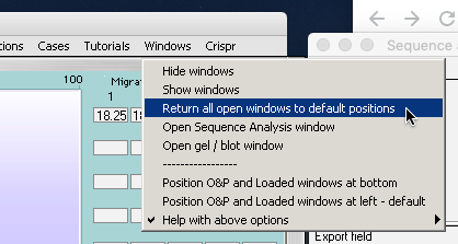
=> Occasionally the lanes may lose their alignment on the gel background, especially when dragging the gel window or the main window on your computer’s desktop. To get them back in the correct locations, use the Windows menu at the top of the Data Screen, and select Return all open windows to default positions.
29. The virtual gel combines lanes from Figures 1B and 1D of Jinek et al. 2012. Compare your gel with Figures 1B and 1D and answer the following questions.
Your Loaded window should look like the one below (the left edge was dragged to expand the window).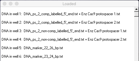
Questions:
A. Why do we only want to show fragments radiolabelled on the 5′ end, in terms of the goal of this particular experiment?
B. Which lanes in Figure 1B and 1D correspond to lanes in the virtual gel?
C. What insights into Cas9 function are apparent from the results of this experiment? How does this function differ for complementary versus non-complementary DNA sequences? Use the markers in lanes 5 and 6 of your gel to help make this determination. (Note: Markers are bands of known size useful for comparison purposes. The computer simulation also allows you to click on any band to reveal its size. The size in bp will appear in the field below the gel).
30. Re-run the above oligonucleotide analyses using the protocol in steps 17-29 above, but this time use DNA oligonucleotides containing protospacer 4. Here are the files and settings that should be used:
DNA: ‘DNA ps 4 comp labelled 5′ end.txt’ and ‘DNA ps 4 non-comp labelled 5′ end.txt’
Enzymes: ‘Cas9 protospacer 1.txt’, ‘Cas9 protospacer 2.txt’, and ‘Cas9 protospacer 4.txt’
[Agarose]: 2.0%
Gel timer: Change the default time of 60 to 45, to keep all fragments on the gel
No marker files will be used for this protospacer 4 experiment (see below).
Note: You end up with 6 lanes for both experiments. The first experiment (using DNA with protospacer 2) had two marker lanes plus 4 lanes for digested DNA. since both the complementary and noncomplementary oligonucleotides were digested by 2 different enzymes. The second experiment (using DNA protospacer 4) will have 6 lanes for digested DNA, since both the complementary and noncomplementary oligonucleotides are digested by 3 different enzymes. No markers are used for our second experiment, as they were in Fig S5B of the original experiment, so you will need to determine the sizes of gel bands by clicking on them. The size in bp will appear in the lower field of the Data Screen.
Compare your results with Figures S3C and S5B, in the Supplement to Jinek et al. 2012, then answer the questions below:
Your Loaded window should look like the one below (the left edge was dragged to expand the window). ![]()
Questions:
A. Why were the experiments repeated using protospacer 4 as a recognition site for Cas9?
B. Do experiments using protospacer 4 give the same results as those involving protospacer 2? Are there any differences between the two sets of results, and if so, how can these be explained in terms of Cas9 function?
C. What additional experiments might be performed to examine the function of Cas9 in more detail?
Top of this page
Go to Part 2: Experiments with mutations to determine Cas9 gene function.
Go to Part 3: PAM requirements and the sensitivity of Cas9 to mismatch
Go to Part 4: Experiments targeting GFP gene sequences